google sheets: a way to analyze data
|
Google Sheets is the Google equivalent of Excel. Google Sheets can do everything Excel can do, plus more. Google Sheets has incredible Add-Ons you can use and, again, the power of collaboration.
Please watch the videos below to see how to use Sheets. |
|
google sheets tutorial
Please watch the video below to learn how to use Google Sheets
tutorial task 1 for google sheets
|
Open up your Google Sheets with your Responses from your Google Form located in your Drive.
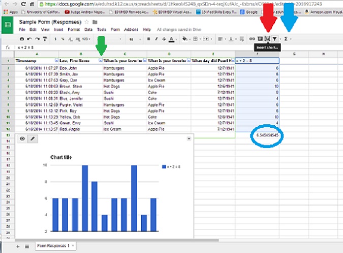
Insert a Graph 1. Insert a graph using the data from your multiple choice question with numerical answers. - Pick the column with the data and highlight it just like you would in an Excel. - Click on the Chart icon as noted by the RED arrow. - Pick the type of chart that you want. - When the graph appears grab it and position it where you would like. Insert a Formula 1. Click on the open cell beneath the numbers (Blue circle in the example). - Click on the Formula icon (Blue arrow in example). - Pick the formula you want and click it. - Highlight the cells you want included in the calculation. 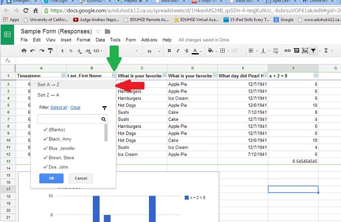
|
Sort a Field
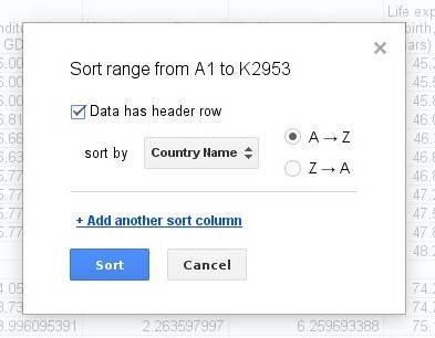
1. Go to the column with your student names and sort them in alphabetical order. 2. Click on the arrow next to the title of that column (Green arrow in the example). - Pick how you want to sort the column (Red Arrow). - Hit OK and the column will be resorted just like in Excel. |
TUTORIAL TASK 2 FOR GOOGLE SHEETS
|
TUTORIAL: USING GOOGLE SHEETS
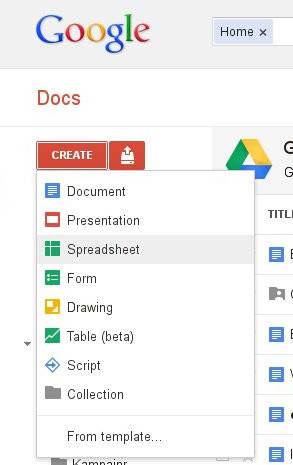
Creating a Sheet and Importing Data Introduction: The most basic tool used for data wrangling is a spreadsheet. Data contained in a spreadsheet is in a structured, computer-readable format and hence can quickly be sorted, filtered, and manipulated (calculated, counted, …). Walkthrough: Creating a Spreadsheet and uploading data.
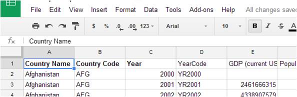
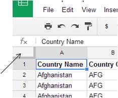
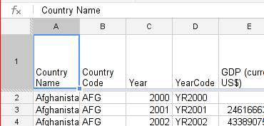
Navigating and using the Spreadsheet Now that you have loaded some data let’s deal with the basics of spreadsheets. A spreadsheet is basically a table of “cells” in which you can input data. The cells are organized in “rows” and “columns”. Typically rows are labeled by numbers, columns by letters. This also means cells can be addressed by their “column” and “row” coordinates. The cell A1 denotes the cell in the first row in the first column, A2 the one in the second row, B1 the one in the second column and so on. To enter or change data in a cell click on it and start typing – this will change the contents of the cell. Walkthrough: Formating 1. Make all the titles in the first row (Country, Country Code …) on the spreadsheet bold by clicking the cell then clicking on the bold button (see image) 2. Adjust the columns to fit your data. A. Select all the data by clicking the blank box in the upper left of the grid. (see image) B. Click on the FORMAT menu then click on WRAP TEXT C. You can also adjust the width of a column or height of a row by moving the cursor between columns or rows until you see a two sided arrow. Click and drag the column or row to make it bigger or smaller. You can also double click on the line between columns and row and it will automatically adjust the width or height. Basic navigation can be done more efficiently via the keyboard. A list of keyboard shortcuts good to know below: Key or Combination What it does Tab End input on the current cell and jump to the cell right to the current one Enter End input and jump to the next row (This will try to be intelligent, so if you’re entering multiple columns, it will jump to the first column you are entering) Up Move to the cell one row up Down Move to the cell one row down Left Move to the cell left Right Move to the cell on the Right Ctrl+<direction> Move to the outermost cell in the direction given Shift+<direction> Select the current cell and the cell in <direction> Ctrl+Shift+<direction> Select all cells from the current to the outermost cell in <direction> Ctrl+c Copy – copies the selected cells into the clipboard Ctrl+v Paste – pastes the clipboard Ctrl+x Cut – copies the selected cells into the clipboard and removes them from their original position Ctrl+z Undo – undoes the last change you made Ctrl+y Redo – undoes an undo Crtl+f Find - useful for searching within the spreadsheet Tip: Practice a bit, and you will find that you will become a lot faster using the keyboard than the mouse! Locking Rows and Columns The spreadsheet we are working on is quite large. You will notice, that while scrolling the column with the column labels will frequently disappear, leaving you quite lost. The same with the country names. To avoid this you can “lock” rows and columns so they don’t disappear. Walkthrough: Locking the top row
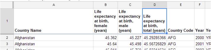
The first thing to do when looking at a new dataset is to orient yourself. This involves at looking at maximum/minimum values and sorting the data so it makes sense. Let’s look at the columns. We have data about the GDP, healthcare expenditure and life expectancy. Now let’s explore the range of data by simply sorting. Your Assignment: You have been asked to investigate the average life expectancy of females and males from different countries using the data from the World Bank (this is the same data in your spreadsheet). Walkthrough: Moving Columns or Rows 1. Move the cursor over the columns at the top of the spreadsheet and left click over the “J.” Only this column is now selected and should be highlighted blue. The cursor should now be an opened hand (if not, move the cursor to the center of the cell). 2. Hold the left click button in (the hand will now close) and drag the entire column over the “B” column then unclick. The data for female life expectancy should now be next to the country name. Notice that the data that was in column B (country code) got bumped over one column and is not deleted. 3. Move the data for male life expectancy (now in column K) and total life expectancy to columns C and D. (see image) Sorting Walkthrough: Sorting a dataset
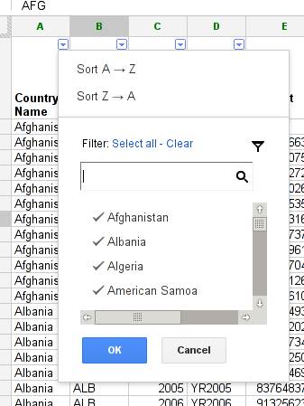
Filtering Data The next thing commonly done with datasets is to filter out the values you don’t want to see. Did you notice that some “Country Names” are actually not countries? You’ll find things like “World”, “North America” and “Arab World”. Let’s filter them out. Walkthrough: Filtering Data
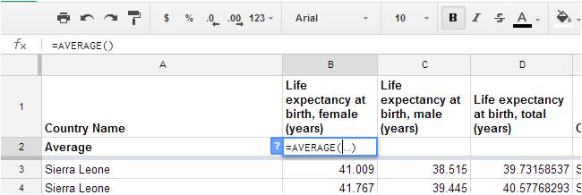
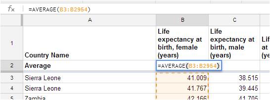
Now it is time for some additional analysis of the data. What is the average life expectancy for females and males for countries with data in your spreadsheet? This is the real power of a spreadsheet. Imagine entering all this data into a calculator. Using calculations and functions (Google)/formulas (Microsoft) not only saves time it also makes automatic adjustments if the data is changed. Walkthrough: Adding a Row or Column 1. Click on the row heading (the numbers on the side of the spreadsheet) that you would like to insert a row below. For your data, click the “1” and the row of heading will highlight. 2. Click the INSERT menu then ROW BELOW and a new row will appear. 3. Lock that row in place (remember how to do it? If not look at the directions above for locking rows and columns). Functions (Formulas) Spreadsheets can be used to count and calculate data in just about every way. The key inputting the correct function/formula for what you are looking for. Each function/formula in a spreadsheet starts with the equal sign “=”. If you are familiar with the function/formula you can simply type it in. For example: =sum(B2:B5) will total what is in cells B2 through B5. =sum(B2+B5) will add cell B2 to B5. Common functions/formulas are found in the FUNCTIONS MENU (see image). Click on this button to bring up a list of common functions. Walkthrough: Inserting a Function (Formula) 1. Click Cell A2 and type the title AVERAGE. Notice that without an equal sign “=” the spreadsheet knew this was text and not a formula. 2. Click in cell B2 (below Life Expectancy for females). Click the FUNCTIONS MENU (sigma sign) then AVERAGE. (see image) 3. To define the range of data to average, highlight all the data in column B from B3 downward. You may also type the range B3:B2954 (that is the range of your data). See image. 4. Press enter and the average is now calculated! Walkthrough: Copying a Function (Formula) 1. To apply this calculation to the Life Expectancy of Males, simply select the cell with the function you wish to copy (in your spreadsheet it is B2). It will now have a blue border. 2. You can copy then paste using the EDIT menu (or keyboard shortcut) to the open cell C2. The spreadsheet will adjust the function automatically to average the data in column C. 3. Another way to copy the function is to select the cell with the function (B2 or C2), carefully move the cursor to the lower right of the blue border until it is a large +. Click and hold, then drag the across the cells you wish to apply the formula (they will be bordered with a dashed line). When you release the function will automatically apply. Link to Google Sheets Working with Functions Further Reading and References
Modified from School of Data website: http://schoolofdata.org/handbook/courses/sort-and-filter/ |


|
ways in which you can use google sheets with your students
* Collect data from a lab or from a survey and have your students analyze the data in a group or small pairs
* Sort data gathered from your students or parents in Google Forms
* Sort data gathered from your students or parents in Google Forms
